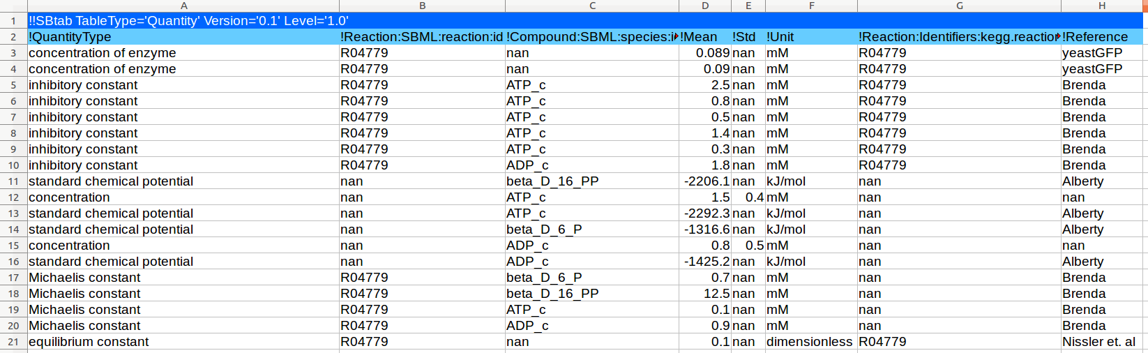
| Standard chemical potential |
μ0 |
kJ/mol |
Species |
Additive |
Thermodynamic |
Basic |
0 |
500 |
|
-500 |
500 |
10 |
|
Global parameter |
1 |
[I_species, 0, 0, 0, 0, 0, 0, 0] |
| Catalytic rate constant geometric mean |
kV |
1/s |
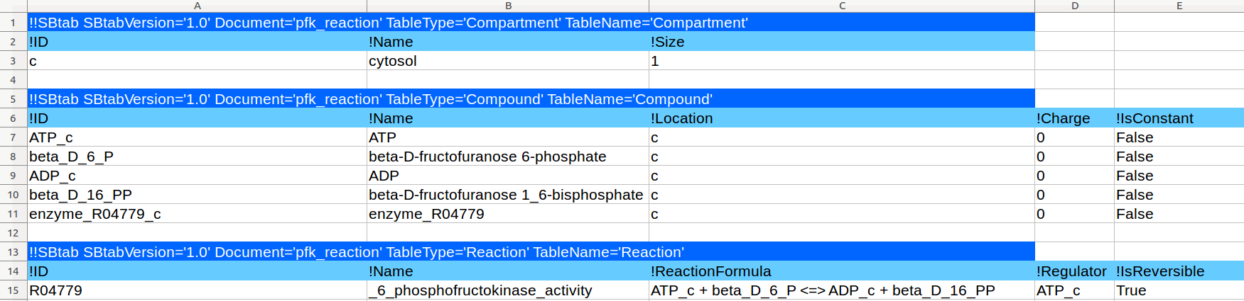
Reaction |
Multiplicative |
Kinetic |
Basic |
10 |
|
100 |
0.00000001 |
10000 |
10 |
1.2 |
Local parameter |
1 |
[0, I_reaction, 0, 0, 0, 0, 0, 0] |
| Michaelis constant |
kM |
mM |
Reaction/Species |
Multiplicative |
Kinetic |
Basic |
0.1 |
|
10 |
0.0000001 |
1000 |
1 |
1.2 |
Local parameter |
1 |
[0, 0, I_KM, 0, 0, 0, 0, 0] |
| Activation constant |
kA |
mM |
Reaction/Species |
Multiplicative |
Kinetic |
Basic |
0.1 |
|
10 |
0.0001 |
100 |
1 |
1.2 |
Local parameter |
1 |
[0, 0, 0, I_KA, 0, 0, 0, 0] |
| Inhibitory constant |
kI |
mM |
Reaction/Species |
Multiplicative |
Kinetic |
Basic |
0.1 |
|
10 |
0.0001 |
100 |
1 |
1.2 |
Local parameter |
1 |
[0, 0, 0, 0, I_KI, 0, 0, 0] |
| Concentration |
c |
mM |
Species |
Multiplicative |
Dynamic |
Basic |
0.1 |
|
10 |
0.0000001 |
1000 |
1 |
1.2 |
Species (conc.) |
1 |
[0, 0, 0, 0, 0, I_species, 0, 0] |
| Concentration of enzyme |
u |
mM |
Reaction |
Multiplicative |
Dynamic |
Basic |
0.001 |
|
100 |
0.0000001 |
0.5 |
0.05 |
1.2 |
Local parameter |
1 |
[[-1/RT * Nt], 0, 0, 0, 0, 0, 0, 0] |
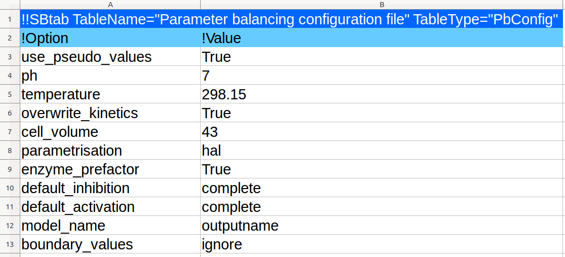
| pH |
pH |
dimensionless |
None |
Additive |
Dynamic |
Basic |
7 |
1 |
|
0 |
14 |
1 |
|
Global parameter |
1 |
[0, 0, 0, 0, 0, 0, 0, 1] |
| Standard Gibbs energy of reaction |
dmuO |
kJ/mol |
Reaction |
Additive |
Thermodynamic |
Derived |
0 |
500 |
|
-1000 |
1000 |
10 |
|
Global parameter |
0 |
[Nt, 0, 0, 0, 0, 0, 0, 0] |
| Equilibrium constant |
keq |
dimensionless |
Reaction |
Multiplicative |
Thermodynamic |
Derived |
1 |
|
100 |
0.00000000001 |
10000000000 |
10 |
1.2 |
Local parameter |
1 |
[[-1/RT * Nt], 0, 0, 0, 0, 0, 0, 0] |
| Substrate catalytic rate constant |
kcat+ |
1/s |
Reaction |
Multiplicative |
Kinetic |
Derived |
10 |
|
100 |
0.01 |
1000000000 |
10 |
1.2 |
Local parameter |
1 |
[[-0.5/RT * Nt], I_reaction, [-0.5 * Nkm], 0, 0, 0, 0, 0] |
| Product catalytic rate constant |
kcat- |
1/s |
Reaction |
Multiplicative |
Kinetic |
Derived |
10 |
|
100 |
0.00000000001 |
1000000000 |
10 |
1.2 |
Local parameter |
1 |
[[0.5/RT * Nt], I_reaction, [0.5 * Nkm], 0, 0, 0, 0, 0] |
| Chemical potential |
μ |
kJ/mol |
Species |
Additive |
Dynamic |
Derived |
0 |
500 |
|
-500 |
500 |
10 |
|
|
0 |
[I_species, 0, 0, 0, 0, [RT * I_species], 0, 0] |
| Reaction affinity |
A |
kJ/mol |
Reaction |
Additive |
Dynamic |
Derived |
0 |
500 |
|
-100 |
100 |
10 |
|
|
0 |
[[-1 * Nt], 0, 0, 0, 0, [-RT * Nt], 0, 0] |
| Forward maximal velocity |
vmax+ |
mM/s |
Reaction |
Multiplicative |
Dynamic |
Derived |
0.01 |
|
100 |
0.000000001 |
10000000 |
0.1 |
2 |
Local parameter |
0 |
[[-0.5/RT * Nt], I_reaction, [-0.5 * Nkm], 0, 0, 0, I_reaction, 0] |
| Reverse maximal velocity |
vmax- |
mM/s |
Reaction |
Multiplicative |
Dynamic |
Derived |
0.01 |
|
100 |
0.000000001 |
10000000 |
0.1 |
2 |
Local parameter |
0 |
[[0.5/RT * Nt], I_reaction, [0.5 * Nkm], 0, 0, 0, I_reaction, 0] |
| Forward mass action term |
thetaf |
1/s |
Reaction |
Multiplicative |
Dynamic |
Derived |
1 |
|
1000 |
0.000000001 |
100000000 |
1 |
2 |
|
0 |
[[-1/(2*RT) * h * Nt], I_reaction, - 1/2 * h * abs(Nkm), 0, 0, h * Nft, 0, 0] |
| Reverse mass action term |
thetar |
1/s |
Reaction |
Multiplicative |
Dynamic |
Derived |
1 |
|
1000 |
0.000000001 |
100000000 |
1 |
2 |
|
0 |
[[ 1/(2*RT) * h * Nt], I_reaction, - 1/2 * h * abs(Nkm), 0, 0, h * Nrt, 0, 0] |
| Forward enzyme mass action term |
tauf |
mM/s |
Reaction |
Multiplicative |
Dynamic |
Derived |
1 |
|
1000 |
0.000000001 |
100000000 |
1 |
2 |
|
0 |
[[-1/(2*RT) * h * Nt], I_reaction, - 1/2 * h * abs(Nkm), 0, 0, h * Nft, I_reaction, 0] |
| Reverse enzyme mass action term |
taur |
mM/s |
Reaction |
Multiplicative |
Dynamic |
Derived |
1 |
|
1000 |
0.000000001 |
100000000 |
1 |
2 |
|
0 |
[[ 1/(2*RT) * h * Nt], I_reaction, - 1/2 * h * abs(Nkm), 0, 0, h * Nrt, I_reaction, 0] |
| Michaelis constant product |
KMprod |
mM |
Reaction |
Multiplicative |
Kinetic |
Derived |
1 |
1000 |
|
0.001 |
1000 |
1 |
2 |
Local parameter |
0 |
[0, 0, Nkm, 0, 0, 0, 0, 0] |
| Catalytic constant ratio |
Kcatratio |
dimensionless |
Reaction |
Multiplicative |
Kinetic |
Derived |
1 |
|
10 |
0.00000000001 |
10000000000 |
1 |
2 |
Local parameter |
0 |
[-1/RT * Nt], I_reaction, [-1 * Nkm], 0, 0, 0, 0, 0] |